Basic image operation
- 이번 장 에서는 이미지에 다양한 효과를 줄 수 있는 이미지 연산 방법에 대하여 알아보겠습니다.
- 이미지로 할 수 있는 기본 연산을 총 네 가지로 나누어서 설명하겠습니다. 각각의 기본 연산들을 조합해서 훨씬 더 많은 효과를 낼 수 있습니다.
- 네 가지 기본 연산은 아래와 같습니다.
Import Libraries
import os
import sys
import math
from platform import python_version

import cv2
import matplotlib.pyplot as plt
import matplotlib

import numpy as np

print("Python version : ", python_version())
print("Opencv version : ", cv2.__version__)
matplotlib.rcParams['figure.figsize'] = (4.0, 4.0)
Python version :  3.6.9
Opencv version :  4.1.2
Data load
sample_image_path = '../image/'
sample_image = 'kitten.jpg'
img = cv2.imread(os.path.join(sample_image_path, sample_image), cv2.IMREAD_GRAYSCALE)
h, w = img.shape
Data description
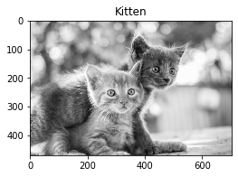
- 본 예제에서 사용할 데이터는 아래와 같습니다.
plt.imshow(img, cmap='gray')
plt.title('Kitten')
plt.show()
Dot operation
- Dot Operation이란, Source Image의 Pixel과 Target Image의 Pixel간의 1:1 연산을 말합니다.
- 이것을 수식으로는 아래와 같이 표현할 수도 있습니다.
- $pixel(i, j)_{after} = f(pixel(i, j)_{before})$
- 여기에서 다시 함수 $f$에 따라 Affine[2] , Gamma[3] 연산으로 나눌 수 있습니다.
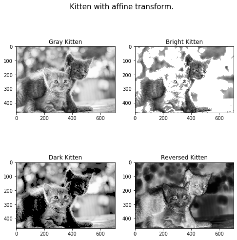
- 아래 코드는 몇 가지 Affine Operation 예시 입니다.
bright_img = img + 50
bright_img[img > 155] = 255
dark_img = img - 50
dark_img[img < 100] = 0
reverse_img = 255 - img

plt.figure(figsize=(8, 8))
plt.subplot(2, 2, 1)
plt.imshow(img, cmap='gray')
plt.title('Gray Kitten')

plt.subplot(2, 2, 2)
plt.imshow(bright_img, cmap='gray')
plt.title('Bright Kitten')

plt.subplot(2, 2, 3)
plt.imshow(dark_img, cmap='gray')
plt.title('Dark Kitten')

plt.subplot(2, 2, 4)
plt.imshow(reverse_img, cmap='gray')
plt.title('Reversed Kitten')

plt.suptitle('Kitten with affine transform.', size=15)
plt.show()
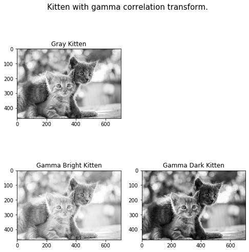
- 아래 코드는 Gamma Correlation Operation 예시 입니다.
bright_gamma = 0.5
dark_gamma = 1.5
bright_gamma_image = np.uint8(255 * np.power(img / 255, bright_gamma))
dark_gamma_image = np.uint8(255 * np.power(img / 255, dark_gamma))

plt.figure(figsize=(8, 8))
plt.subplot(2, 2, 1)
plt.imshow(img, cmap='gray')
plt.title('Gray Kitten')

plt.subplot(2, 2, 3)
plt.imshow(bright_gamma_image, cmap='gray')
plt.title('Gamma Bright Kitten')

plt.subplot(2, 2, 4)
plt.imshow(dark_gamma_image, cmap='gray')
plt.title('Gamma Dark Kitten')

plt.suptitle('Kitten with gamma correlation transform.', size=15)
plt.show()
- Gamma Correlation Transform과 Affine Transform이 각각 Image에 끼치는 영향이 어떤 차이가 있을까요?
- 변환된 각 Image의 Histogram을 확인해보면 차이를 확실히 알 수 있습니다.
def histogram_cv(img):
    h, w = img.shape[:2]
    hist = cv2.calcHist([img], [0], None, [256], [0, 256])
    hist = hist / (h * w)
    return hist
plt.figure(figsize=(12, 8))

plt.subplot(2, 3, 1)
plt.imshow(img, cmap='gray')
plt.title('Kitten')

plt.subplot(2, 3, 2)
plt.imshow(bright_img, cmap='gray')
plt.title('Affine bright Kitten')

plt.subplot(2, 3, 3)
plt.imshow(bright_gamma_image, cmap='gray')
plt.title('Gamma bright Kitten ')

plt.subplot(2, 3, 4)
plt.plot(histogram_cv(img))
plt.title('Kitten Histogram')

plt.subplot(2, 3, 5)
plt.plot(histogram_cv(bright_img))
plt.title('Affine bright Kitten Histogram')

plt.subplot(2, 3, 6)
plt.plot(histogram_cv(bright_gamma_image))
plt.title('Gamma bright Kitten Histogram')

plt.suptitle('Histogram comparison', size=15)
plt.show()
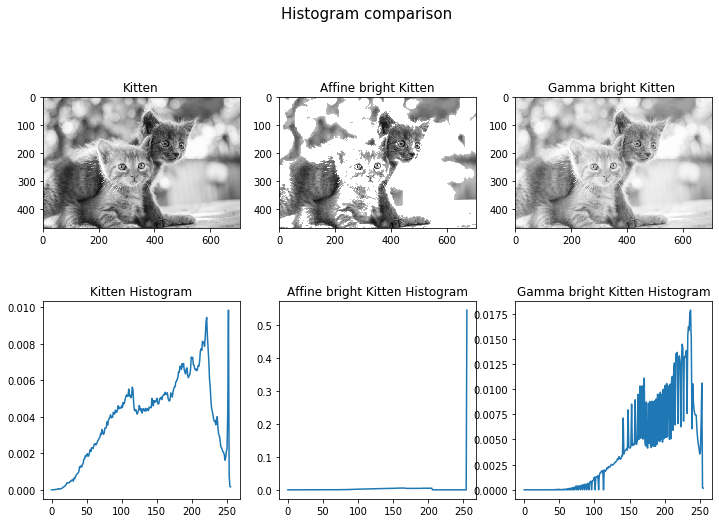
- 원래 Image와 변환된 Image들의 Histogram 입니다.
- Affine 변환의 경우 픽셀값에 상수를 더하여 밝게 만들고, 픽셀값의 최대치인 255에 도달하면 그냥 255에 놔두는 반면,
- Gamma Correlation 변환의 경우 히스토그램의 분포 형태를 어느 정도 유지하며 밝아지는 모습을 확인할 수 있습니다.
- 이 두 연산의 차이는 그림과 히스토그램을 같이 볼 때 더 크게 체감이 됩니다. Affine Operation을 적용한 경우, 가장 밝은 부분부터 뭉개지는 듯한 모습인 반면, Gamma Operation을 적용할 경우 원래 형태를 유지하며 밝아지는 모습입니다.
Area operation
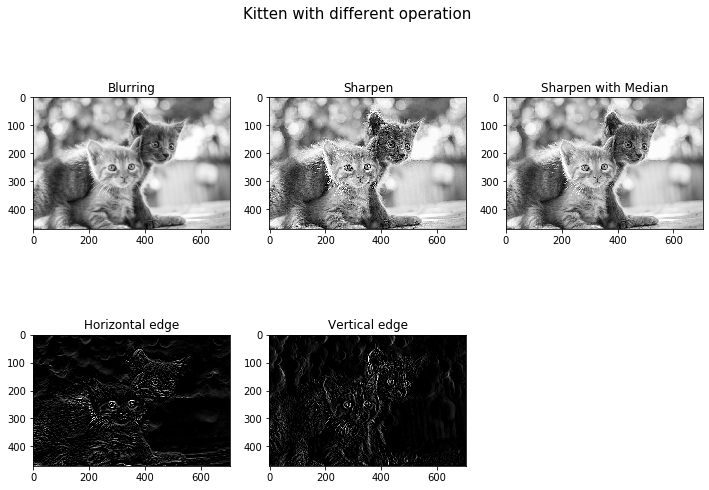
- Area Operation이란, Target Image의 한 Pixel값을 결정하기 위해 Source Image의 여러 개의 Pixel값을 필요로 하는 연산을 말합니다.
- Source Image의 여러 Pixel값들에 특정 가중치를 부여하고, Source Image와 가중치의 곱의 합을 구하여 Target Image를 구하는 방법이 일반적 입니다.
- 여기에서 특정 가중치를 구할 때, 일정한 크기의 Mask에만 유효한 값을 부여하고 나머지 영역에는 0을 부여하곤 합니다.
- 이러한 연산을 Correlation, 혹은 Convolution이라고 합니다.
- Correlation과 Convolution은 엄밀히 말하면 서로 다른 연산이나, Image Processing의 특성상 거의 같은 연산인 것으로 생각하고 넘어가겠습니다.
- OpenCV에서 ‘cv2.filter2D()’ 를 통해 쉽게 적용할 수 있고, 몇몇 자주 쓰이거나 특별한 연산의 경우 따로 정의된 함수가 존재하기도 합니다.
- (e.g)Median Filter[4] 는 ‘cv2.medianBlur(img,kernel)’ 을 통해 제공되는데, 엣지 정보를 잘 남겨두면서 노이즈를 제거하는 방법으로 알려져 있습니다.
- 어떠한 Mask를 사용하느냐에 따라 결과 영상의 특성이 천차 만별로 달라질 수 있습니다.
- 아래 예시중 수평, 수직방향 Edge를 각각 구한 결과가 있습니다. 예시에서 사용된 Mask가 Sobel Filter의 초기 모델이며, Edge Detection에서 자세히 다루겠습니다.
- Sharpen이라는 기법은 물체의 Edge를 강하게 드러내는 방법중 하나 입니다.
- 위 연산들은 앞서 말했다시피 완전히 다른 결과를 만들지만, 적용하는 Mask만 다를 뿐 같은 함수 호출을 통해 만들어낸 결과임을 주목합시다.
blur_mask = np.ones((3, 3), dtype=np.uint8) / 9
horiz_edge_mask = np.array([[1, 1, 1],
                            [0, 0, 0],
                            [-1, -1, -1]])
vert_edge_mask = np.array([[1, 0, -1],
                           [1, 0, -1],
                           [1, 0, -1]])
sharp_mask = np.array([[0, -1, 0],
                      [-1, 5, -1],
                      [0, -1, 0]])

dst1 = cv2.filter2D(img, -1, blur_mask)
dst2 = cv2.filter2D(img, -1, horiz_edge_mask)
dst3 = cv2.filter2D(img, -1, vert_edge_mask)
dst4 = cv2.filter2D(img, -1, sharp_mask)
dst4_blur = cv2.medianBlur(dst4, 3)

plt.figure(figsize=(12,8))
plt.subplot(231)
plt.imshow(dst1, cmap='gray')
plt.title('Blurring')

plt.subplot(232)
plt.imshow(dst4, cmap='gray')
plt.title('Sharpen')

plt.subplot(233)
plt.imshow(dst4_blur, cmap='gray')
plt.title('Sharpen with Median')

plt.subplot(234)
plt.imshow(dst2, cmap='gray')
plt.title('Horizontal edge')

plt.subplot(235)
plt.imshow(dst3, cmap='gray')
plt.title('Vertical edge')

plt.suptitle('Kitten with different operation', size=15)
plt.show()
Geometric operation
- 세 번째 Geometric Operation은 영상에 이동, 크기, 회전, 기울임 등의 효과를 주는 것을 말합니다.
- 물체의 기하학적 특징이 탄력적으로 보존되는 변환입니다.
- 찢거나 구기거나 흐릿하게 만들거나 하지 않고, 눈 두개 사이에 코가 있다는 등의 특성이 기울어지든, 회전하든 그대로 유지된다는 의미로 받아들이시면 됩니다.
- 4가지 기본적인 연산을 순차적으로 조합하여 수 많은 변환을 수행할 수 있습니다[5].
- e.g. 특정 점을 기준으로 회전, 좌우 반전(Flip), 시점 변환(Perspective transform) 등
- OpenCV에서 지원하는 ‘cv2.getAffineTransform()’, ‘cv2.warpAffine()’ 함수를 통해 Geometric Operation을 적용할 수 있습니다.
- 여기에서 함수 이름에 들어가는 Affine 때문에 헷갈리는 경우가 있을 수 있을 것 같습니다.
- Dot Operation에서 소개한 Affine Operation은 개별 픽셀값 하나에 대한 Affine연산이며, 여기에서 나온 Affine의 의미는 Image의 전체 픽셀들에 대하여 지역적으로 적용하는 Affine 연산입니다.
- 이 둘의 차이는, 어떤 픽셀에 대하여 그 ‘값’을 바꾸느냐, 혹은 그 ‘위치’를 바꾸느냐에 따라 나뉘는 것으로 생각하시면 되겠습니다.
pts1 = np.float32([[50, 50], [200, 50], [50, 200]])
pts2 = np.float32([[10, 100], [200, 50], [100, 250]])

M = cv2.getAffineTransform(pts1, pts2)
dst1 = cv2.warpAffine(img, M, (w, h))

M = cv2.getRotationMatrix2D((w / 2, h / 2), -30, 1)
dst2 = cv2.warpAffine(img, M, (w, h))

plt.figure(figsize=(12, 4))
plt.subplot(1, 3, 1)
plt.imshow(img, cmap='gray')
plt.title('Input')

plt.subplot(1, 3, 2)
plt.imshow(dst1, cmap='gray')
plt.title('Affine')

plt.subplot(1, 3, 3)
plt.imshow(dst2, cmap='gray')
plt.title('Rotation')

plt.suptitle('Lena with geometric transform')
plt.show()
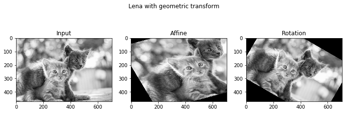
- 간단하게 고양이 Image를 뒤틀고, 회전시켜본 예시입니다.
- 각 함수의 자세한 사용법은 OpenCV 공식 문서[6]에서 확인할 수 있습니다.
Interpolation
- Image의 크기를 바꾸는 경우(특히 확대할 때), 원본 Image의 픽셀과 픽셀 사이에 새로운 값이 생성되는 것이므로 이 새로운 값을 어떻게 채워야 할 지에 대한 문제가 발생하게 됩니다.
- 단순하게 한 쪽 픽셀 값을 그대로 가져다가 적용할 경우 영상이 실질적으로 해상도가 커지는 것이 아니라, 단순히 크기만 키우는 것 이라고 볼 수 있습니다.
- 이와 반대로 (머신러닝 등의 방법 없이)더 좋은 해상도의 Image를 얻기 위하여 Interpolation을 사용합니다.
- OpenCV는 다양한 Interpolation(보간법)을 제공하는데, ‘cv2.resize()’ 함수의 인자 ‘interpolation’ 으로 조절할 수 있습니다.
- ‘cv2.INTER_NEAREST’ - 최근접 이웃 픽셀의 값을 사용함. (size의 단순한 확대)
- ‘cv2.INTER_LINEAR’ - 양 선형 보간 (default 값)
- ‘cv2.INTER_AREA’ - 영역의 넓이에 기반한 방법. (사이즈를 줄일 때 좋은 성능)
- ‘cv2.INTER_CUBIC’ - 양 3차 보간 : 양 선형 보간법 보다 4배 많은 정보를 활용.
- ‘cv2.INTER_LANCZOS4’ - Lanczos 보간 : 양 3차 보간법 보다 4배 많은 정보를 활용.
h, w = [int(x) for x in img.shape]
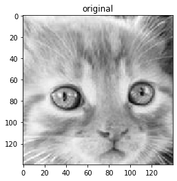
face_img = img[h // 2 - 60 : h // 2 + 80, w // 2 - 110 : w // 2 + 30]
h, w = [int (x) for x in face_img.shape]
dst3 = np.zeros([h * 2, w * 2])
for i in range(h):
for j in range(w):
dst3[2 * i, 2 * j] = face_img[i, j]
dst3[2 * i + 1, 2 * j + 1] = face_img[i, j]
dst3[2 * i, 2 * j + 1] = face_img[i, j]
dst3[2 * i + 1, 2 * j] = face_img[i, j]
dst4 = cv2.resize(face_img, (w * 2, h * 2))
dst5 = cv2.resize(face_img, (w * 2, h * 2), interpolation=cv2.INTER_CUBIC)
dst6 = cv2.resize(face_img, (w * 2, h * 2), interpolation=cv2.INTER_LANCZOS4)
plt.figure(figsize=(4, 4))
plt.imshow(face_img, cmap='gray')
plt.title('original')
plt.show()
plt.figure(figsize=(16, 16))
plt.subplot(2, 2, 1)
plt.imshow(dst3, cmap='gray')
plt.title('resize manual')

plt.subplot(2, 2, 2)
plt.imshow(dst4, cmap='gray')
plt.title('resize bilinear')

plt.subplot(2, 2, 3)
plt.imshow(dst5, cmap='gray')
plt.title('resize cubic')

plt.subplot(2, 2, 4)
plt.imshow(dst6, cmap='gray')
plt.title('resize lanczos4')
plt.show()
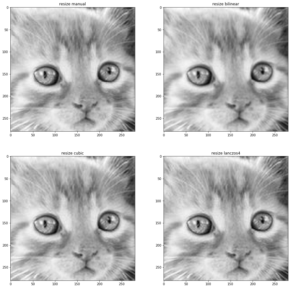
- 아기 고양이의 얼굴만 확대한 Image를 통해 Interpolation 방법에 따른 Image 품질 차이를 확인해보겠습니다.
- Manual Resize된 Image와 Interpolation이 적용된 Image와의 품질 차이는 확실히 드러납니다.
- 나머지 Interpolation이 적용된 Image들의 품질을 여러분의 눈으로는 확인 가능하신가요? 자세히 보시면 보일겁니다.
- Bilinear Interpolation은 새로운 픽셀의 값을 계산할 때 양 옆의 두 픽셀만을 고려하기 때문에 계산량이 다소 적은 편 입니다.
- Cubic, Lanczos4 등의 방법론은 더 많은 주변 픽셀들을 고려하기 때문에 일반적으로 Bilinear보다 더 높은 품질의 결과물을 보여줍니다.
- 연산 효율이 중요할 경우에는 bilinear interpolation을, 결과물의 품질이 중요한 경우에는 Cubic이나 Lanczos4중에서 선택하시면 됩니다.
Conclusion
- Image에 적용하는 기본 연산들을 알아보았습니다.
- 원하는 효과를 내기 위해 다양한 방식으로 연산을 조합해서 눈으로 직접 확인해보시면 많은 도움이 될 것 입니다.
Reference
- [1] 오일석, “영상 처리의 세 가지 기본 연산,” in 컴퓨터 비전, vol.4, Republic of Korea:한빛아카데미, 2014, pp. 76-92
- [2] Accessed: ‘Affine transformation’, Wikipedia. 2019 [Online]. Available: https://en.wikipedia.org/wiki/Affine_transformation
- [3] Accessed: ‘Gamma correction’, Wikipedia. 2019 [Online]. Available: https://en.wikipedia.org/wiki/Gamma_correction
- [4] Accessed: ‘Median filter’, Wikipedia. 2019 [Online]. Available: https://en.wikipedia.org/wiki/Median_filter
- [5] Accessed: ‘Denavit–Hartenberg parameters’, Wikipedia. 2019 [Online]. Available: https://en.wikipedia.org/wiki/Denavit%E2%80%93Hartenberg_parameters
- [6] Accessed: ‘Geometric Image Transformations’, ‘OpenCV 2.4.13.7 documentation’. 2019 [Online]. Available: https://docs.opencv.org/2.4/modules/imgproc/doc/geometric_transformations.html
- [7] Accessed: ‘Free Cat, Kitten Adoptions In Anne Arundel’, Patch. 2018 [Online]. Available: https://patch.com/maryland/annearundel/free-cat-kitten-adoptions-anne-arundel