[Tutorial] Image Thresholding

Introduction

• OpenCV와 Python으로 Image processing을 알아봅시다.
• 이 글에서는 Image thresholding을 간단히 알아보고, 어떻게 응용되는지 Blob labeling예제를 통해 확인하겠습니다.

Import Libraries

import os
import sys
import math
from platform import python_version

import cv2
import matplotlib.pyplot as plt
import matplotlib
import numpy as np

print("Python version : ", python_version())
print("OpenCV version : ", cv2.__version__)
matplotlib.rcParams['figure.figsize'] = (4.0, 4.0)

Python version :  3.6.7
OpenCV version :  3.4.5

Data load

sample_image_path = '../image/'
sample_image = 'lena_gray.jpg'
img = cv2.imread(sample_image_path + sample_image, cv2.IMREAD_GRAYSCALE)

coin_image = 'coins.jpg'
mask = np.array([[0, 1, 0],[1, 1, 1], [0, 1, 0]], dtype=np.uint8)
coin_img = cv2.imread(sample_image_path + coin_image, cv2.IMREAD_GRAYSCALE)

ret, coin = cv2.threshold(coin_img, 240, 255, cv2.THRESH_BINARY_INV)
coin = cv2.dilate(coin, mask, iterations=1)
coin = cv2.erode(coin, mask, iterations=6)

Data description

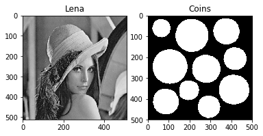
• 본 예제에서 사용할 데이터는 아래와 같습니다.
  • Lena : 지난 예제에서 사용한 Lena 입니다.
  • Coins : Blob labeling 예제에서 사용될 이미지 입니다.
    • blob labeling이라는 주제에 맞게 전처리가 된 이미지 입니다. (blob labeling에서 자세하게 설명합니다.)

plt.subplot(1, 2, 1)
plt.imshow(img, cmap='gray')
plt.title('Lena')
plt.subplot(1, 2, 2)
plt.imshow(coin, cmap='gray')
plt.title('Coins')
plt.show()

Binarization

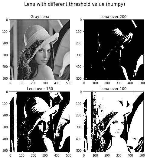
• Binarization(이진화)이란, grayscale의 이미지를 기준에 따라 0 또는 1의 값만을 갖도록 만드는 작업입니다.
  • 일반적으로 특정 픽셀 값을 기준으로 더 작은 값은 0으로, 더 큰 값은 1로 만듭니다.
  • 사용 목적에 따라 결과 값을 반전시킬 때도 있는데, 추후에 코드 예시로 알아보겠습니다.
• 이진화 자체는 단순한 작업이나, 추후에 보다 발전된 알고리즘을 다루기 위한 기본이 됩니다.

def simple_img_binarization_npy(img, threshold):
    w, h = img.shape
    b_img = np.zeros([w, h])
    b_img[img > threshold] = 1
    return b_img

plt.figure(figsize=(8, 8))
b_img1 = simple_img_binarization_npy(img, 200)
b_img2 = simple_img_binarization_npy(img, 150)
b_img3 = simple_img_binarization_npy(img, 100)

plt.subplot(2, 2, 1)
plt.imshow(img, cmap='gray')
plt.title('Gray Lena')

plt.subplot(2, 2, 2)
plt.imshow(b_img1, cmap='gray')
plt.title('Lena over 200')

plt.subplot(2, 2, 3)
plt.imshow(b_img2, cmap='gray')
plt.title('Lena over 150')

plt.subplot(2, 2, 4)
plt.imshow(b_img3, cmap='gray')
plt.title('Lena over 100')

plt.suptitle('Lena with different threshold value (numpy)', size=15)
plt.show()

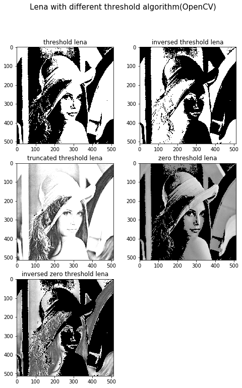
• 위에서 numpy를 이용했다면, 이번엔 OpenCV 내장 함수를 이용하여 image threshold를 해보겠습니다.
• OpenCV 함수를 이용하면 numpy로 작성하는 것 보다 편리하게 다양한 결과물을 만들어낼 수 있습니다.
  • cv2.threshold() 함수에 전달하는 인자를 통해 threshold 알고리즘을 다양하게 변경할 수 있습니다.

ret, thresh1 = cv2.threshold(img, 127, 255, cv2.THRESH_BINARY)
ret, thresh2 = cv2.threshold(img, 127, 255, cv2.THRESH_BINARY_INV)
ret, thresh3 = cv2.threshold(img, 127, 255, cv2.THRESH_TRUNC)
ret, thresh4 = cv2.threshold(img, 127, 255, cv2.THRESH_TOZERO)
ret, thresh5 = cv2.threshold(img, 127, 255, cv2.THRESH_TOZERO_INV)

plt.figure(figsize=(8, 12))
plt.subplot(3, 2, 1)
plt.imshow(thresh1, cmap='gray')
plt.title('threshold lena')

plt.subplot(3, 2, 2)
plt.imshow(thresh2, cmap='gray')
plt.title('inversed threshold lena')

plt.subplot(3, 2, 3)
plt.imshow(thresh3, cmap='gray')
plt.title('truncated threshold lena')

plt.subplot(3, 2, 4)
plt.imshow(thresh4, cmap='gray')
plt.title('zero threshold lena')

plt.subplot(3, 2, 5)
plt.imshow(thresh5, cmap='gray')
plt.title('inversed zero threshold lena')

plt.suptitle('Lena with different threshold algorithm(OpenCV)', size=15)
plt.show()

Otsu Algorithm

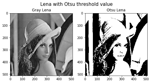
• Otsu algorithm(오츄 알고리즘)은 특정 threshold값을 기준으로 영상을 둘로 나눴을때, 두 영역의 명암 분포를 가장 균일하게 할 때 결과가 가장 좋을 것이다는 가정 하에 만들어진 알고리즘입니다.
  • 여기서 균일함 이란, 두 영역 각각의 픽셀값의 분산을 의미하며, 그 차이가 가장 적게 하는 threshold 값이 오츄 알고리즘이 찾고자 하는 값입니다.

• 위에 기술한 목적에 따라, 알고리즘에서는 특정 Threshold $T$를 기준으로 영상을 분할하였을 때, 양쪽 영상의 분산의 weighted sum이 가장 작게 하는 $T$값을 반복적으로 계산해가며 찾습니다.

  • weight는 각 영역의 넓이로 정합니다.
  • 어떤 연산을 어떻게 반복하는지에 대한 내용이 아래 수식에 자세히 나와있습니다.
    $$ \begin{align} & T = argmin_{t\subseteq {1,\cdots,L-1}} v_{within}(t) \\
    & v_{within}(t) = w_{0}(t)v_{0}(t) + w_{1}(t)v_{1}(t) \\
    \\
    & w_{0}(t) = \Sigma_{i=0}^{t} \hat h(i),\hspace{2cm} && w_{1}(t) = \Sigma_{i=t+1}^{L-1} \hat h(i)\\
    & \mu_{0}(t)=\frac{1}{w_{0}(t)}\Sigma_{i=0}^{t}i\hat h(i) && \mu_{1}(t)=\frac{1}{w_{1}(t)}\Sigma_{i=t+1}^{L-1}i\hat h(i)\\
    & v_{0}(t) = \frac{1}{w_{0}(t)}\Sigma_{i=0}^{t}i\hat h(i)(i-\mu_{0}(t))^2 && v_{1}(t) = \frac{1}{w_{1}(t)}\Sigma_{i=t+1}^{L-1}i\hat h(i)(i-\mu_{1}(t))^2\\
    \end{align} $$

• $w_{0}(t), w_{1}(t)$는 threshold 값으로 결정된 흑색 영역과 백색 영역의 크기를 각각 나타냅니다.

• $v_{0}(t), v_{1}(t)$은 두 영역의 분산을 뜻합니다.

• 위 수식을 그대로 적용하면 시간복잡도가 $\Theta(L^{2})$이므로 실제로 사용하기 매우 어려워집니다.

• 그러나, $\mu$와 $v$가 영상에 대해 한번만 계산하고 나면 상수처럼 취급된다는 사실에 착안하여 다음 알고리즘이 완성되었습니다.
  $$ \begin{align} &T = argmax_{t\subseteq{0,1,\cdots,L-1}}v_{between}(t)\\
  &v_{between}(t)=w_{0}(t)(1-w_{0}(t))(\mu_{0}(t)-\mu_{1}(t))^2\\
  &\mu = \Sigma_{i=0}^{L-1}i\hat h(i)\\
  \\
  &\text{초깃값}(t=0):w_{0}(0)=\hat h(0),\ \mu_{0}(0)=0\\
  &\text{순환식}(t>0):\\
  & \hspace{1cm} w_{0}(t)=w_{0}(t-1)+\hat h(t)\\
  & \hspace{1cm} \mu_{0}(t)=\frac{w_{0}(t-1)\mu_{0}(t-1)+t\hat h(t)}{w_{0}(t)}\\
  & \hspace{1cm} \mu_{1}(t)=\frac{\mu-w_{0}(t)\mu_{0}(t)}{1-w_{0}(t)}\\
  \end{align} $$

• 위 순환식을 $t$에 대하여 수행하여 가장 큰$v_{between}$를 갖도록 하는 $t$를 최종 threshold $T$로 사용합니다.

• 이와 같은 알고리즘이 OpenCV의 threshold함수에 구현되어있으며, cv2.THRESH_OTSU 파라미터를 아래 코드와 같이 사용하면 적용이 됩니다.

plt.figure(figsize=(8, 4))
ret, th = cv2.threshold(img, 0, 255, cv2.THRESH_BINARY + cv2.THRESH_OTSU)

plt.subplot(1, 2, 1)
plt.imshow(img, cmap='gray')
plt.title('Gray Lena')

plt.subplot(1, 2, 2)
plt.imshow(th, cmap='gray')
plt.title('Otsu Lena')

plt.suptitle('Lena with Otsu threshold value', size=15)
plt.show()

Blob labeling

• Threshold를 통해 할 수 있는 일은 그야말로 무궁무진한데, 그 중 하나로 이미지 분할(image segmentation)을 예시로 들 수 있습니다.

  • 만일 threshold 등의 알고리즘을 이용하여 특정 목적에 따라 영상을 분할할 수 있다면(e.g. 사람 손 or 도로의 차선) 1로 정해진 픽셀끼리 하나의 object라고 생각할 수 있을것이고, 우리는 이 object를 묶어서 사용하고 싶게 될 것입니다.

• 서로 다른 object인지를 판단하기 위하여 픽셀의 연결성 [2] 을 고려한 알고리즘을 수행하고 각기 다른 label을 할당하는데, 이를 Blob labeling이라 합니다.

• Blob labeling을 하면 개별 object에 대해 각각 접근하여 우리가 하고싶은 다양한 영상처리를 개별적으로 적용할 수 있게 되니, 활용도가 아주 높은 기능입니다.

  • 본 예제에서는 blob labeling에 대한 개념적인 소개와 OpenCV에 구현된 함수의 간단한 사용법을 확인하겠습니다. [3]
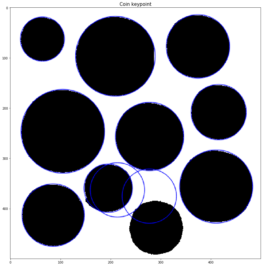
  • 직관적으로 원의 형상을 띄는 위치에 하나의 blob을 의미하는 파랑색 동그라미를 생성하는 모습입니다.
  • 잘못된 위치에 그려진 blob이 눈에 띄는데요, 이와 같은 결과를 parameter를 통해 handling하는 내용에 대해서 차후 다가올 주제인 Image Segmentation에서 확인하겠습니다.

ret, coin_img = cv2.threshold(coin, 200, 255, cv2.THRESH_BINARY_INV)

params = cv2.SimpleBlobDetector_Params()
params.minThreshold = 10
params.maxThreshold = 255
params.filterByArea = False
params.filterByCircularity = False
params.filterByConvexity = False
params.filterByInertia = False

detector = cv2.SimpleBlobDetector_create(params) # Blob detector 선언
keypoints = detector.detect(coin_img)  # Blob labeling 수행
im_with_keypoints = \
cv2.drawKeypoints(coin_img, keypoints, np.array([]), (0, 0, 255),
                  cv2.DRAW_MATCHES_FLAGS_DRAW_RICH_KEYPOINTS)  # 원본 이미지에 찾은 blob 그리기

plt.figure(figsize=(15,15))
plt.imshow(im_with_keypoints)
plt.title('Coin keypoint', size=15)
plt.show()

Conclusion

• Image thresholding의 사용법과 다양한 응용방법, threshold 값을 선택해주는 Otsu 알고리즘을 알아보았습니다.
• 마지막에 알아본 Blob labeling은 Image processing 분야 전반에 걸쳐 사용되는 곳이 아주 많으니 추후에 더 깊이 알아보는 시간을 갖겠습니다.

Reference

• [1] 오일석, 컴퓨터 비전, 2014, pp. 67-75
• [2] ‘Pixel connectivity’, Wikipedia. 2019 [Online]. Available: https://en.wikipedia.org/wiki/Pixel_connectivity
• [3] Satya Mallick., ‘Blob Detection Using OpenCV ( Python, C++ )’, ‘Learn OpenCV. 2019 [Online]. Available: https://www.learnopencv.com/blob-detection-using-opencv-python-c/